About CO-NO2 Metal Oxide Sensors¶

The SGX Mics is a Metal Oxide Resistive sensor capable of reacting to different substances in the atmosphere. In a simplified way, it is comprised of two main elements:

A SnO₂ substrate that acts as a sensor element
A heater element to keep the substrate in an optimal working area

The SnO₂ is a chemically sensitive metal oxide which has interactions with molecules to be detected in the target gas. The reactions that can occur on SnO₂ surface are adsorption and catalytic reactions, which basically mean that the gas molecules can be adsorbed onto the surface or can catalyse reactions (trigger or enhance them). They take place at the so called active sites or grain boundaries, which are areas where the grains that constitute the sensor resistance are in contact with the air (e.g. with metallic contacts). Hence, metal oxide substrate is basically a collection of sites at which different molecules can be absorbed and therefore interact in various manners with the species present in the atmosphere: either through catalytic reaction, surface reaction, grain boundary reaction (among others). ².

The sensor element is typically heated to a few hundred degrees (ºC) using a small resistive heater. The regions within the sensor can be described as in Peterson et al. ¹: the surface, which interacts with the gas, the bulk, which is unaffected by it, and the particle boundary, which lies in between these two. The particle boundary is situated at a distance from any material exposed to the atmosphere into the sensor that chemical electrostatic effects can propagate (the so called Debye length), and this is related to the material’s physical properties. At high temperatures, oxygen atoms bond onto the boundary, extracting electrons in the process from the semiconductor’s surface region. The oxygen either then directly reacts with ambient gases, or these gases also bond onto the sensor, which causes more charge carriers to be withdrawn or injected into the surface region. All these effects change the sensor resistance and it is measured accordingly in ¹:

In the case of the SGX 4514, the detection of the pollution gases is achieved by measuring the sensing resistance of both sensors. In a generic way, we could characterise the sensor resistance as follows:

RED sensor resistance decreases in the presence of CO and hydrocarbons.
OX sensor resistance increases in the presence of NO₂.

Finally, the chemical reactions within the resistive element are directly related to temperature and follow an Arrhenius equation type of behaviour. Each sensor's type has a different optimal operation temperature, which is translated into different heating powers for the heater element. Depending on the heating power and transition speeds, different reactions can be facilitated and this can lead to positive effects such as sensor clean up or battery compsuption savings, for example, when heated up in a pulsed profile. On the other hand, it can facilitate sensor poisoning or ageing, which highlights the need of proper sensor characterisation.

Sensor Calibration¶

The SGX4514 is a low cost sensor originally ment to detect instances or trends of target gas in the atmosphere ⁴⁵. The applications intended for these sensors are ‘event sensing‘ applications and the level of accuracy required is not necessarily within regulatory standards. Furthermore, these sensors should not be used with safety related issues.

However, despite the low cost nature of these sensors, they have been subject of a great deal of research ¹²³ and have been reported to give considerably good results in field applications. Before delving into the details of sensor calibration, we will try to understand what these sensors are and how they should be handled. Some important definitions are:

Sensor baseline resistance: is the resistance that the sensor exhibits when it's not powered
Sensor sensitivity: is the resistance variation with variations in the target gas
Sensor cross-sensitivity: is the resistance variation with variations of gases other than the target gas
Sensor poisoning: an irreversible resistance variation provoked by the reaction of gases other than the target gas

Source: Peterson et al. ¹

Peterson et al. ¹ describes the various types of interactions between atmospheric gases and a MOS sensor surface. In the image above, the leftmost region describes the unpowered behaviour, or base resistance. The three other regions of the diagram describe different processes that actually occur simultaneously to varying degrees. The sensor’s output is the resistance across the whole of the sensor material, which forms a resistor network with contributions from both the bulk and surface regions. The model described in ¹ also explains the wide variation in base resistance between individual sensors of the same type, as the random nature of the surface geometry means an equally random network of resistances. This diagram is a two-dimensional representation of a three-dimensional material; in an actual sensor, the sensitive region is spread into the surface with a distance dependent on the grain size and arrangement resulting from the sintering.

Each sensor will then have a different resistance in air and how much this baseline resistance changes with the concentration of the target gas will also differ (what we defined above as sensitivity). Therefore to convert from resistance readings to concentration it is necessary to derive a calibration curve for each sensor. This will require measuring the resistances in air and at a number of gas concentrations over the desired range. It is important that the concentrations are in a background of air as Oxygen is needed for the sensor to work correctly. As stated in ², the sensor’s response is only partially a function of the amount of gas to which the surface is exposed. Instead, the sensor will have a baseline resistance that is related to the bulk and particle boundary resistance. Because of the random geometry of the granular sensor surface, the baseline resistance will vary between individual sensors.

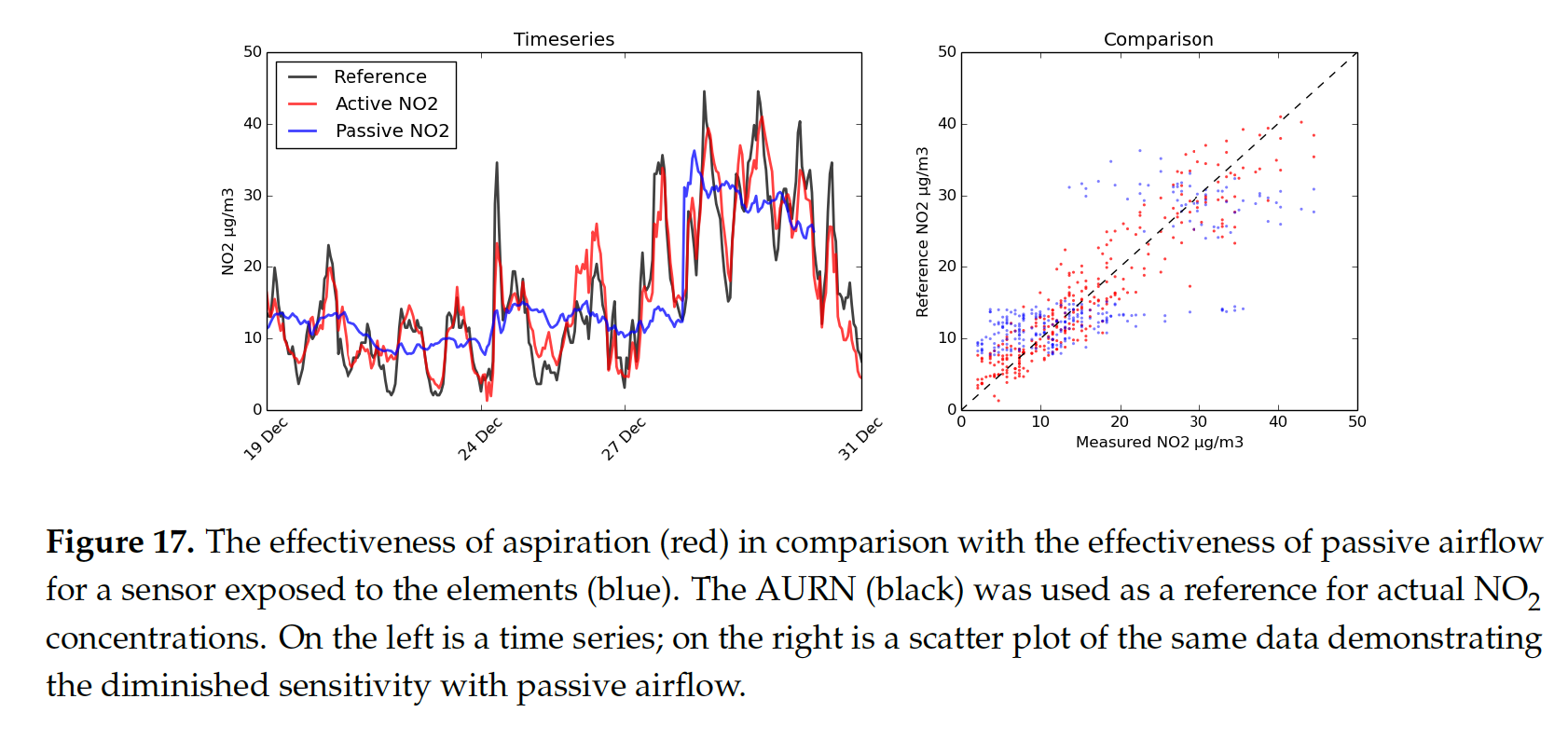
The change in resistance with the change in gas concentration is generally not a linear response. The response can be measured and fitted to a polynomial relationship, with interactions from other metrics such as temperature, humidity and other gases. It has been proved that air flow around the sensor yields better sensor reactivity, and that the usage of PTFE filters also helps reducing cross-sensitivity and sensor poisoning. An important practical consideration with any in situ air quality sensor design is ensuring adequate flow of sampling air through the device. Stale air inside a casing will produce unrepresentative results, and even sensors mounted outside a casing might not get a properly-mixed sample.

Source: Peterson et al. ¹

Although the deployment of multiple different sensors can compensate for the cross-sensitivity issues in calibration, it cannot eliminate it. MOS sensors can thus be used only in situations where any interfering species can either be measured by other means, or they must be calibrated regularly and used in locations where the background varies in concentration slowly compared with the target gases. As well, the sensor drift over time is an important issue that requires sensor recalibration over time.

There are two major factors in the longevity of a sensor’s calibration. The first is the natural degradation of the heater element, which becomes hotter over prolonged use and causes the sensor’s response profile to vary. The second is the effect of slowly-varying interfering gases, which over the course of months shifts the sensor’s baseline. The first problem may have an engineering solution, but the second will involve taking the results of the tests in an artificial atmosphere, identifying the most critical species and either measuring or possibly modelling their likely concentrations during deployments.

An analytical approach to counteracting this drift might be "merging calibrations", where a sensor is calibrated at the start and end of a four-month campaign, and the coefficients gradually change from one end of the experiment run to the other.

Having all this in mind, the sensor calibration we follow is comprised of the following steps:

Sensor behaviour characterisation under different temperature profiles
Sensor baseline and sensitivity characterisation in controlled conditions
Sensor deployment with reference measurements collocation and model calibration

The use of deployment campaigns is of utmost importance in order to develop sensor models that are reality proof. With the possibility of collecting the data with the SmartCitizen Platform and the data treatment provided by the Sensor Calibration Framework, we are able to iterate over the different sensor calibration possibilities, ranging from Ordinary Linear Regression or more advanced techniques such as ML models such as LSTMs networks.

Field results¶

In this section, we will detail some of the MOS related results obtained during the sensor validation campaigns detailed below:

University of Bologna: data collected from 23/January to 13/February. The measured pollutants with reference equipments were CO, NO₂, NO, NOx and O3. Two prototype Smart Citizen Stations were deployed in two different sites, with two Smart Citizen Kits.
University College Dublin: data collected from 27/March to 17/April. The measured pollutants with reference equipments were NO, NO₂ and NOX. One prototype Smart Citizen Station was deployed with two Smart Citizen Kits

For both results shown below, we used an LSTM with 200 epochs training and the following structure:

from keras.models import Sequential
from keras.layers import Dense, Activation, LSTM, Dropout

model = Sequential()
layers = [50, 100, 1]
model.add(LSTM(layers[0], return_sequences=True, input_shape=(train_X.shape[1], train_X.shape[2])))
model.add(Dropout(0.2))
model.add(LSTM(layers[1], return_sequences=False))
model.add(Dropout(0.2))
model.add(Dense(output_dim=layers[2]))
model.add(Activation("linear"))
model.compile(loss='mse', optimizer='rmsprop')

Carbon Monoxide¶

The CO model included the following features: $CO_{R}^{-1}$ , $CO_R^{-2}$ , $Temp$ and $Temperature^2$ . The results can be seen below:

Nitrogen Dioxide¶

The NO₂ model included the following features: $NO~2~_{R}$ , $NO~2~_R^{-2}$ , Light, $Temp$ and $Temperature^2$ . The results can be seen below:

Warning

This test campaign contains a short amount of data to be used as a training dataset for a LSTM algorithm. Therefore, this is just to considered as an use case example and further tests and data should be carried out to train broader models.

Metal Oxide Sensors Implementation¶

Heating stage¶

The solution present at Urban Sensor Board V2.0 for MICS-4514 sensor's heaters excitation, pretends to make it compatible with a 3.3V global voltage source.

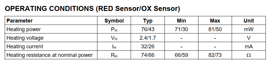
The manufacturer reccomend the following circuit topology, with a global supply voltage of 5V. In the datasheet are collected the electrical nominal conditions for that resistors, in order to operate safely with the heater, without damaging it.

Besides that, several other possible conditions could also damage early the heater resistors, like the fact of consider a pure PWM signal, with source 5V and subsequent dutty cycle, as excitation. Even if the frequency is relatively high (100kHz), the resistors are forced to operate briefly with 5V, and this accelerates the destruction of this part of the MICS sensor.

So its is possible to provide the nominal voltages for heater resistors from a 3.3V source, if we replace the auxiliar resistors (from recomended topology) with corresponding values, to preserve the total power dissipated and current at same normal operating conditions.

Even more, we can upgrade the function of the auxiliar resistors adding a capacitor to form a passive RC filter. In the DC or continuous operation, the capacitor is fully charged and the current is limited by the auxiliar resistor. In AC or pulsed operation, the capacitor can be selected to remove this AC component, and feed the heater resistor with a nearly constant voltage or at least with small variations (<1%).

The source for the PWM signal must be buffered, because the resistive load of the system demands currents avobe the SAMD21 can supply. For this purpose, the solution selected is to use a digital hex-inverter buffer, which can drive up to 32mA with each output pin, wich we can paralelize to operate under propper safety factor for the buffer.

Simulations¶

The first simulations and given values leads to the selection of the RC components values if we set a PWM frequency around 40 kHz.

To evaluate the R part of the filter, is needed to take into account the output resistance of the hex-inverter buffer.

Prototypes¶

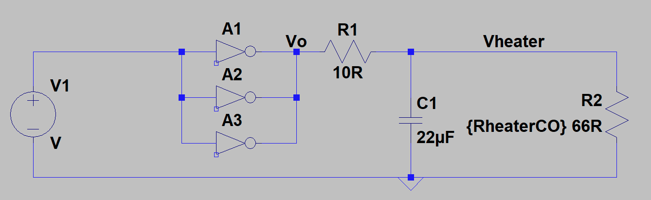
We build the circuit into a protoboard, with several IC HEX-INV manufacturers, based on the following schematic:

The measures are sumarized in the following table, in which we compare four pre-selected devices, which can fit in our application for size an price considerations.

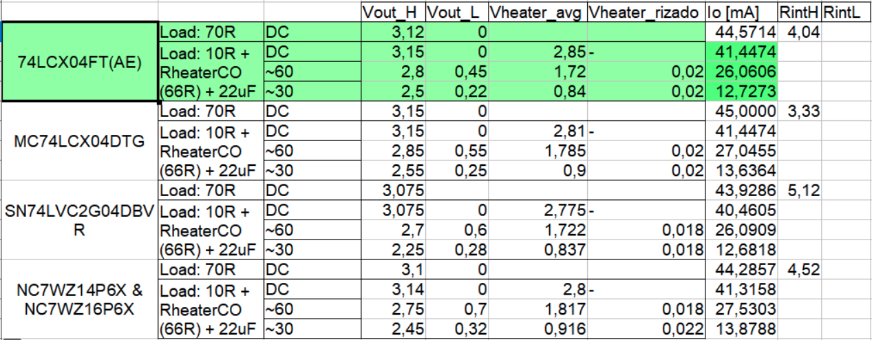
Four cases with paralellized inverters, for each device were performed: pasive load 70R test with DC input, and three tests with 10R+Rheater load at DC input, 60% dutty cycle and 30% dutty cycle. The 74LCX04FT(AE) was selected because it has the lowest LOW output level (0.45V,0.22V), which is considered here as the quality (or close to ideal) of the square wave input source.

Final implementation¶

The solution implemented in the PCB, has a constant auxilar R (10R+Rout_buff), and constant C (47uF), and also operates at consatant frequency, then, the output power regulation is based on the PWM's dutty cycle. The following circuit represent the implemented schematic.

Operation¶

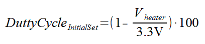
First of all, is needed to know the real implemented Rheater of each sensor (which may vary among devices and time), and can be estimated by measuring the V_heater_* at 100% dutty cycle, then:

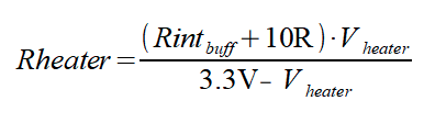
Where Rint_buff can be aproximated with 4 Ohm resistor.

The desired_reference_voltage is function of the desired_power_Rheater and dutty cycle. If we set 80mW we can use the value of the Rheater to obtain desired_reference_voltage through tis formula:

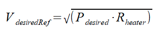
(Take into account this resistor has a drift over time, therefore is recomended to take periodic measurements of the value of Rheater itself, and check the output power reachability).

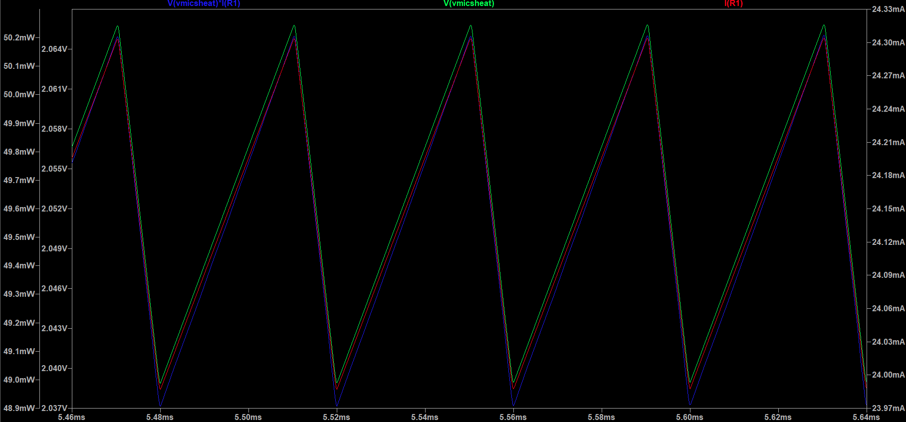
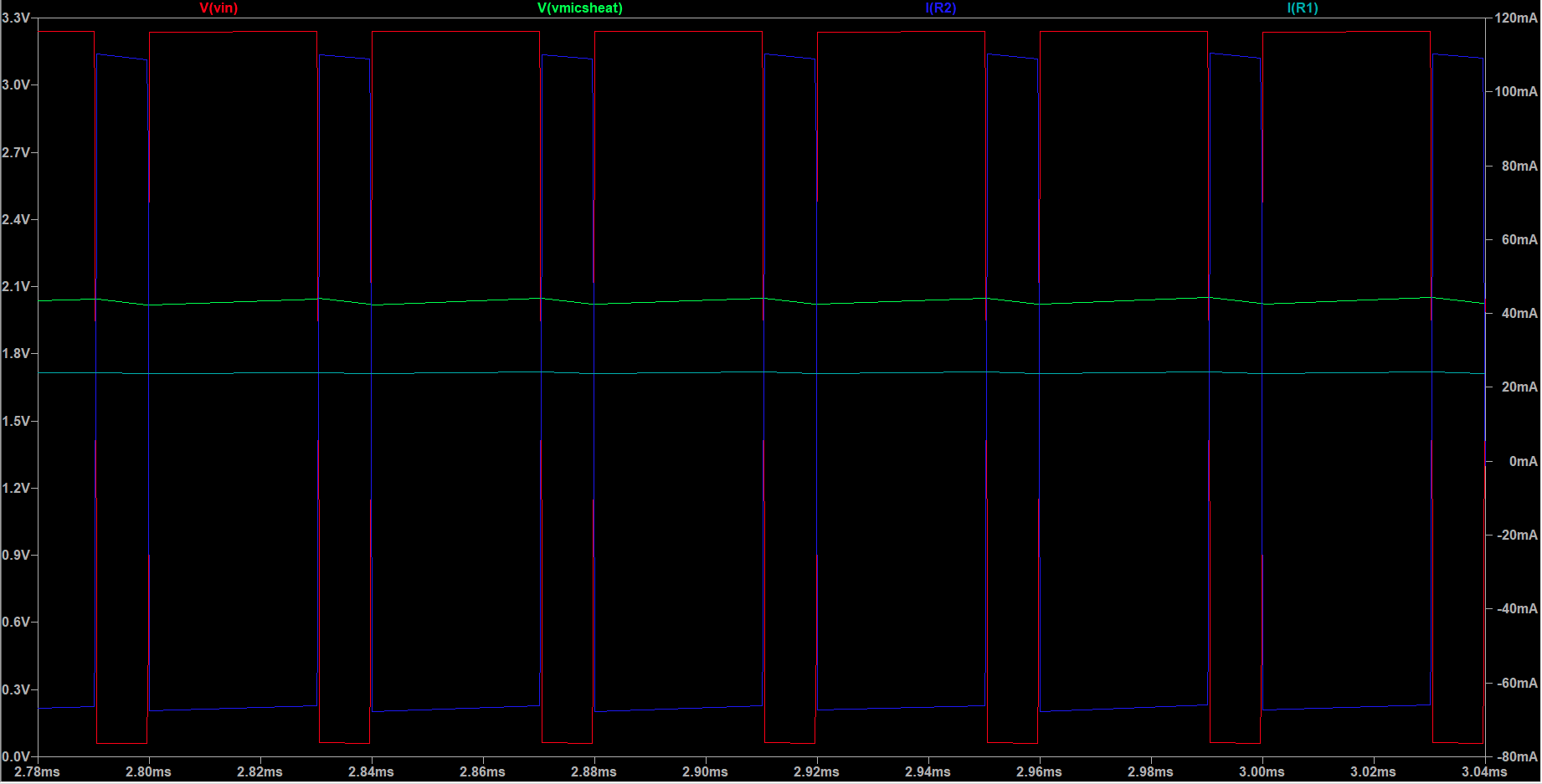
With selected parameters, after 2ms of PWM operation, the RC reaches the permanent, and then is recomended to take measurements of V_HEATER_. The loop can be closed to determine the dutty cycle as function of the difference (desired_reference_voltage – V_HEATER_ (averaged)).

Is recomended to average several samples to remove the AC part of the signal. The measured DC signal has a noise of ±20mV peak to peak (with triangular distribution).

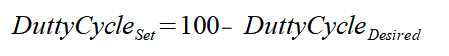
The sign of the PWM signal is inverted due to the action of the inverter, then, a desired x% dutty is obtained as 100%-x%.

As initial PWM aproximation to begin to converge close to the regulated dutty cycle can be obtained through this simplification: