SGX MiCS
The classic Metal Oxyde for CO and NO2 measurements!
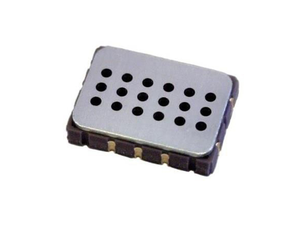
Image Credit: Amphenol SGX Sensortech
Working principle
The SGX Mics is a Metal Oxide Resistive sensor capable of reacting to different substances in the atmosphere. In a simplified way, it is comprised of two main elements:
- A SnO2 substrate that acts as a sensor element
- A heater element to keep the substrate in an optimal working area
The SnO2 is a chemically sensitive metal oxide which has interactions with molecules to be detected in the target gas. The reactions that can occur on SnO2 surface are adsorption and catalytic reactions, which basically mean that the gas molecules can be adsorbed onto the surface or can catalyse reactions (trigger or enhance them). They take place at the so called active sites or grain boundaries, which are areas where the grains that constitute the sensor resistance are in contact with the air (e.g. with metallic contacts). Hence, metal oxide substrate is basically a collection of sites at which different molecules can be absorbed and therefore interact in various manners with the species present in the atmosphere: either through catalytic reaction, surface reaction, grain boundary reaction (among others). 2.
The sensor element is typically heated to a few hundred degrees (ºC) using a small resistive heater. The regions within the sensor can be described as in Peterson et al. 1: the surface, which interacts with the gas, the bulk, which is unaffected by it, and the particle boundary, which lies in between these two. The particle boundary is situated at a distance from any material exposed to the atmosphere into the sensor that chemical electrostatic effects can propagate (the so called Debye length), and this is related to the material’s physical properties. At high temperatures, oxygen atoms bond onto the boundary, extracting electrons in the process from the semiconductor’s surface region. The oxygen either then directly reacts with ambient gases, or these gases also bond onto the sensor, which causes more charge carriers to be withdrawn or injected into the surface region. All these effects change the sensor resistance and it is measured accordingly in 1:
In the case of the SGX 4514, the detection of the pollution gases is achieved by measuring the sensing resistance of both sensors. In a generic way, we could characterise the sensor resistance as follows:
- RED sensor resistance decreases in the presence of CO and hydrocarbons.
- OX sensor resistance increases in the presence of NO2.
Finally, the chemical reactions within the resistive element are directly related to temperature and follow an Arrhenius equation type of behaviour. Each sensor's type has a different optimal operation temperature, which is translated into different heating powers for the heater element. Depending on the heating power and transition speeds, different reactions can be facilitated and this can lead to positive effects such as sensor clean up or battery compsuption savings, for example, when heated up in a pulsed profile. On the other hand, it can facilitate sensor poisoning or ageing, which highlights the need of proper sensor characterisation.
Usage and considerations
Sensor Calibration
The SGX4514 is a low cost sensor originally ment to detect instances or trends of target gas in the atmosphere 45. The applications intended for these sensors are ‘event sensing‘ applications and the level of accuracy required is not necessarily within regulatory standards. Furthermore, these sensors should not be used with safety related issues.
However, despite the low cost nature of these sensors, they have been subject of a great deal of research 123 and have been reported to give considerably good results in field applications. Before delving into the details of sensor calibration, we will try to understand what these sensors are and how they should be handled. Some important definitions are:
- Sensor baseline resistance: is the resistance that the sensor exhibits when it's not powered
- Sensor sensitivity: is the resistance variation with variations in the target gas
- Sensor cross-sensitivity: is the resistance variation with variations of gases other than the target gas
- Sensor poisoning: an irreversible resistance variation provoked by the reaction of gases other than the target gas
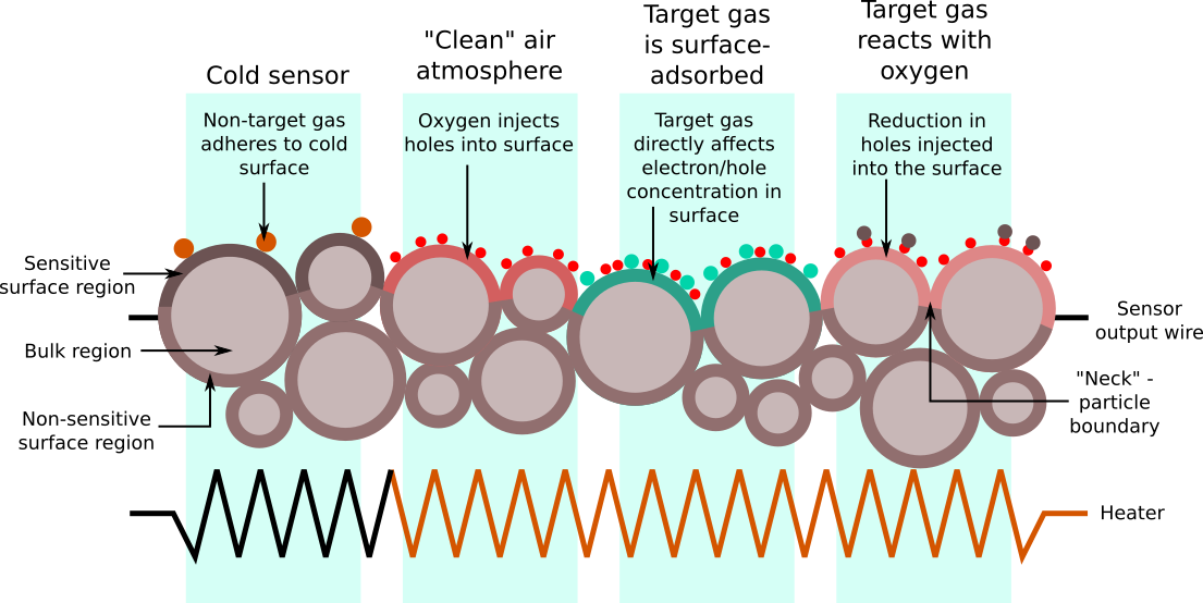 Source: Peterson et al. 1
Peterson et al. 1 describes the various types of interactions between atmospheric gases and a MOS sensor surface. In the image above, the leftmost region describes the unpowered behaviour, or base resistance. The three other regions of the diagram describe different processes that actually occur simultaneously to varying degrees. The sensor’s output is the resistance across the whole of the sensor material, which forms a resistor network with contributions from both the bulk and surface regions. The model described in 1 also explains the wide variation in base resistance between individual sensors of the same type, as the random nature of the surface geometry means an equally random network of resistances. This diagram is a two-dimensional representation of a three-dimensional material; in an actual sensor, the sensitive region is spread into the surface with a distance dependent on the grain size and arrangement resulting from the sintering.
Each sensor will then have a different resistance in air and how much this baseline resistance changes with the concentration of the target gas will also differ (what we defined above as sensitivity). Therefore to convert from resistance readings to concentration it is necessary to derive a calibration curve for each sensor. This will require measuring the resistances in air and at a number of gas concentrations over the desired range. It is important that the concentrations are in a background of air as Oxygen is needed for the sensor to work correctly. As stated in 2, the sensor’s response is only partially a function of the amount of gas to which the surface is exposed. Instead, the sensor will have a baseline resistance that is related to the bulk and particle boundary resistance. Because of the random geometry of the granular sensor surface, the baseline resistance will vary between individual sensors.
The change in resistance with the change in gas concentration is generally not a linear response. The response can be measured and fitted to a polynomial relationship, with interactions from other metrics such as temperature, humidity and other gases. It has been proved that air flow around the sensor yields better sensor reactivity, and that the usage of PTFE filters also helps reducing cross-sensitivity and sensor poisoning. An important practical consideration with any in situ air quality sensor design is ensuring adequate flow of sampling air through the device. Stale air inside a casing will produce unrepresentative results, and even sensors mounted outside a casing might not get a properly-mixed sample.
 Source: Peterson et al. 1
Although the deployment of multiple different sensors can compensate for the cross-sensitivity issues in calibration, it cannot eliminate it. MOS sensors can thus be used only in situations where any interfering species can either be measured by other means, or they must be calibrated regularly and used in locations where the background varies in concentration slowly compared with the target gases. As well, the sensor drift over time is an important issue that requires sensor recalibration over time.
There are two major factors in the longevity of a sensor’s calibration. The first is the natural degradation of the heater element, which becomes hotter over prolonged use and causes the sensor’s response profile to vary. The second is the effect of slowly-varying interfering gases, which over the course of months shifts the sensor’s baseline. The first problem may have an engineering solution, but the second will involve taking the results of the tests in an artificial atmosphere, identifying the most critical species and either measuring or possibly modelling their likely concentrations during deployments.
An analytical approach to counteracting this drift might be "merging calibrations", where a sensor is calibrated at the start and end of a four-month campaign, and the coefficients gradually change from one end of the experiment run to the other.