Sensor calibration
Low-cost sensors give useful information at a fraction of the cost of reference instruments, but their readings are affected by the environment, by other pollutants, by the spread between units and by ageing. Calibration is the process that turns the raw readings of a sensor into values that can be trusted for a given purpose. How much calibration is needed depends on the sensor and on what the data is used for: following trends, comparing locations, or reporting absolute concentrations.
This page explains the general approach, and what it means for each type of sensor we use. The details of each sensor are in its own knowledge page.
Process overview
Typically, sensor calibration requires a series of steps that involve understanding the behaviour of the sensor, to be able to derive a calibration procedure. This process can be split into three stages:
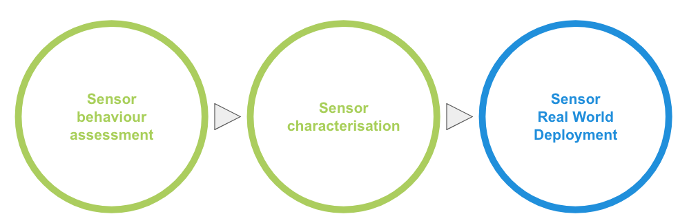
- Behaviour assessment: in laboratory conditions, to assess the general behaviour of the sensor.
- Characterisation: also in laboratory conditions, to find the basic parameters of each sensor.
- Modelling in real world deployments: to account for other variables, such as environmental factors and cross-sensitivity to other pollutants.
Not every sensor goes through every stage, and not every stage is done by us. Many sensors are characterised by their manufacturer, and some even apply corrections internally.
Characterisation
The base calibration parameters are found in controlled conditions:
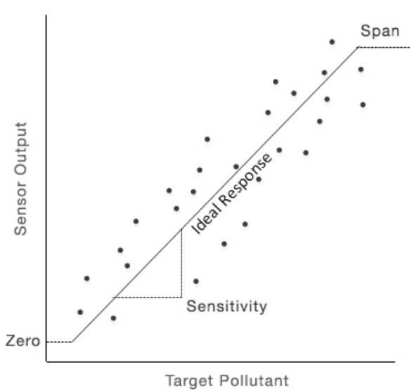
- Sensitivity: the sensor response per unit of the target magnitude (e.g. per ppb of a pollutant) in nominal conditions.
- Zero (or baseline): the sensor reading in zero air, i.e. with none of the target pollutant.
- Response time (t90): the time the sensor takes to reach 90% of its final reading after a step change.
- Range: the minimum and maximum values the sensor can measure.
Field calibration
The conditions in a laboratory can't represent all the conditions found in a real deployment. For this reason, the usual approach is to co-locate the sensors with reference grade instruments (normally, an official air quality monitoring station) for a period of time, and to derive calibration models from the two sets of data 1 2. These models range from simple linear corrections, to multilinear models that include temperature and humidity, to machine learning models 3 4. Some things to keep in mind:
- The models can only be trusted in conditions similar to the ones they were trained with. Co-locations should cover the widest possible range of conditions (seasons, concentrations), and a co-location before and after the deployment is recommended to account for drift 5 6.
- Models can be specific to each sensor and site, or general models derived from several sensors and co-locations, provided that the differences between sensors are small or can be normalised 6.
- More complex models need more data, and they are more prone to learn the artefacts in the data, such as the noise caused by fast changes in temperature and humidity 5.
- The reference data has its own uncertainty: reference stations can deviate up to 15% from the actual concentration 6.
Calibration by sensor type
| Sensor type | Processing | Calibration |
|---|---|---|
| Temperature, humidity, pressure, light, noise | On the sensor | Factory calibration. Offsets can be adjusted |
| Particulate matter | On the sensor | Factory calibration. Field calibration recommended |
| CO2 | On the sensor | Factory calibration and automatic self-calibration |
| Electrochemical sensors | On the platform | Laboratory calibration by the manufacturer. Field calibration recommended |
| Metal oxide sensors | On the sensor | None: indicative only |
| Water sensors | On the sensor | Calibrated by the user with calibration solutions |
Environmental sensors
Temperature, humidity, pressure, light and noise sensors are calibrated by their manufacturer, and their readings are processed on the sensor. The main source of error is not the sensor itself, but the installation: for instance, the temperature inside an enclosure is affected by the heat of the electronics and by solar radiation. Check how to modify the temperature and humidity offsets if needed.
Particulate matter
PM sensors are characterised by the manufacturer, and they calculate the mass concentration internally, assuming the shape, density and optical properties of the particles. Since these assumptions don't hold for every type of aerosol, readings can be over- or underestimated, and a field calibration is needed in almost all cases to report absolute values. High relative humidity makes particles grow by absorbing water, which leads to overestimations, but it can be corrected 7. Check the particulate matter limitations for more details.
CO2
The NDIR CO2 sensors (SCD30 and SCD4X) are calibrated by the manufacturer, and correct their baseline over time with an automatic self-calibration, which assumes that the sensor is exposed to fresh air regularly. When this is not the case, a forced recalibration against a known concentration can be done instead. Check each sensor page for how to do it.
Electrochemical sensors
The Alphasense electrochemical sensors are characterised individually by the manufacturer in laboratory conditions. The firmware only reports the raw voltages of the electrodes, and the concentrations are calculated on the platform using this calibration data, following the Alphasense application notes. For this, the calibration data of each unit needs to be linked to the device.
This processing gives good enough information to start a deployment and follow trends, but it does not account for all the effects of temperature, humidity, other pollutants and ageing in the deployment conditions. When accurate values are needed, a field calibration with a reference station is recommended. Check the data processing section for the details.
Metal oxide sensors
Metal oxide sensors, such as the SGX MICS used in previous versions of the SCK, have a large spread in their baseline resistance and sensitivity between units, a low selectivity to their target pollutant, and drift over time. Even when they are characterised in the laboratory, their behaviour changes during the deployment, which makes their individual calibration unrealistic. Their readings should be taken as indicative only. Check the sensor calibration section of the MICS page for more details.
Water sensors
The Atlas Scientific water sensors need to be calibrated by the user with calibration solutions, before the first use and periodically after that. Check each sensor page: pH, dissolved oxygen, conductivity, ORP and temperature. Soil moisture sensors, such as the Chirp, are calibrated with dry and wet reference points.
Data processing
When a sensor needs processing on the platform, we do it automatically with our default algorithms, for the devices that have it set up. If you want to try different algorithms, you can run them yourself, with the same tools we use. Check the guides on handling calibration data and data processing.
References
-
Clements, A., S. Lung, A. Arfire, AND A. Polidori. An Update on Low-Cost Sensors for the Measurement of Atmospheric Composition: Evaluation Activities. World Meteorological Organization, Geneva, Switzerland, (2020). ↩
-
Spinelle, L., M. Gerboles, M. G. Villani, M. Aleixandre, and F. Bonavitacola. “Field Calibration of a Cluster of Low-Cost Available Sensors for Air Quality Monitoring. Part A: Ozone and Nitrogen Dioxide.” Sensors and Actuators B: Chemical (2015). https://doi.org/10.1016/j.snb.2015.03.031. ↩
-
Hagan, D. H., G. Isaacman-VanWertz, J. P. Franklin, L. M. M. Wallace, B. D. Kocar, C. L. Heald, and J. H. Kroll. “Calibration and Assessment of Electrochemical Air Quality Sensors by Co-Location with Regulatory-Grade Instruments.” Atmospheric Measurement Techniques 11 (2018). https://doi.org/10.5194/amt-11-315-2018. ↩
-
Zimmerman, N., A. A. Presto, S. P. N. Kumar, J. Gu, A. Hauryliuk, E. S. Robinson, A. L. Robinson, and R. Subramanian. “A Machine Learning Calibration Model Using Random Forests to Improve Sensor Performance for Lower-Cost Air Quality Monitoring.” Atmospheric Measurement Techniques 11 (2018). https://doi.org/10.5194/amt-11-291-2018. ↩
-
iSCAPE Project Deliverable 7.8 Sensor monitoring experiences and technological innovations (November 2019). Link ↩↩
-
Node-to-node field calibration of wireless distributed air pollution sensor network. Environmental Pollution (2017). https://doi.org/10.1016/j.envpol.2017.09.042 ↩↩↩
-
Di Antonio, Andrea, Olalekan Popoola, Bin Ouyang, John Saffell, and Roderic Jones. “Developing a Relative Humidity Correction for Low-Cost Sensors Measuring Ambient Particulate Matter.” Sensors 18, no. 9 (August 24, 2018): 2790. https://doi.org/10.3390/s18092790. ↩